Deep NLP - Speech Recognition

Speech recognition (SR) is the inter-disciplinary sub-field of computational linguistics that develops methodologies and technologies that enables the recognition and translation of spoken language into text by computers.

Speech recognition
Neural network speech recognition

Speech recognition

Speech problems

Automatic speech recognition
- Spontaneous vs read speech
- Large vocabulary
- In noise
- Low resource
- Far-field
- Accent-independent
- Speaker-adaptive
Text to speech
- Low resource
- Realistic prosody
Speaker identification
Speech enhancement
Speech separation

Acoustic representation

Speech physical realization

Waves of changing air pressure.
Realised through excitation from the vocal cords
Modulated by the vocal tract.
Modulated by the articulators (tongue, teeth, lips)
Converted to Voltage with a microphone
Sampled with an Analogue to Digital Converter
Human hearing is 50Hz-20kHz
Human speech is 85Hz–8kHz
Contemporary speech processing mostly around 16kHz 16bits/sample

We want a low-dimensionality representation, invariant to speaker, background noise, rate of speaking etc.

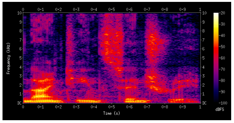
Fourier analysis shows energy in diﬀerent frequency bands
windowed short-term fast Fourier transform (FFT)
e.g. FFT on overlapping 25ms windows (400 samples) taken every 10ms
- Energy vs frequency [discrete] vs time [discrete]
- can hadle it as images

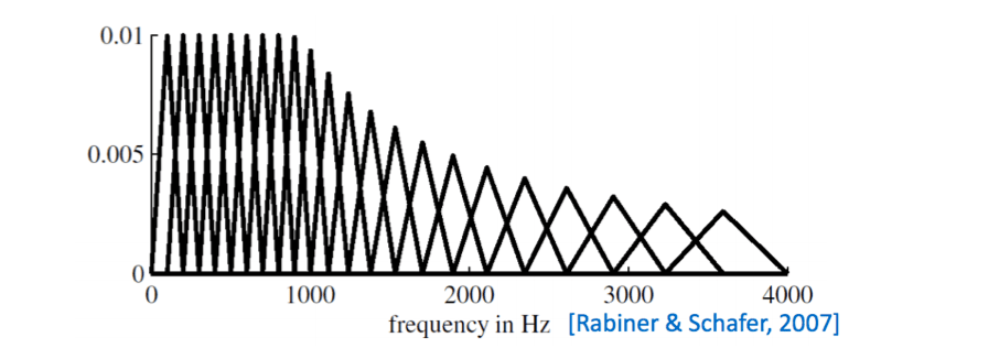
Mel frequency representation

FFT is still too high-dimensional for conventional ASR system
Downsample by local weighted averages on mel scale non-linear spacing, and take a log. \[ m = 1127\ln(1+\frac{f}{700}) \]
Result in log-mel features (default for neural network speech modelling.)
40+ dimensional features per frame

MFCC

Mel Frequency Cepstral Coeﬃcients - MFCCs are the discrete cosine transformation of the mel ﬁlterbank energies. Whitened and low-dimensional.

Similar to Principal Components of log spectra
GMM speech recognition systems may use 13 MFCCs

Perceptual Linear Prediction – a common alternative representation.

Frame stacking- it’s common to concatenate several consecutive frames.

e.g. 26 for fully-connected DNN. 8 for LSTM.

GMMs used local diﬀerences (deltas) and second-order diﬀerences (delta-deltas) to capture dynamics. (13 + 13 + 13 dimensional). Ultimately use 39 dimensional linear discriminant analysis ( class-aware PCA) projection of 9 stacked MFCC vectors.

Phonetic representation

Speech evolved as communication to convey information, consists of sentences (in ASR we usually talk about “utterances”). Sentences composed of words.

Minimal unit is a “phoneme”

Minimal unit that distinguishes one word from another
Set of 40-60 distinct sounds
Vary per language
Universal representations
- IPA: international phonetic alphabet
- X-SAMPA (ASCII)

Homophones

distinct words with the same pronunciation: “there” vs “their”

Prosody

How something is said can convey meaning.

Datasets

TIMIT
- Hand-marked phone boundaries given
- 630 speakers × 10 utterances
Wall Street Journal (WSJ) 1986 Read speech. WSJ0 1991, 30k vocab
Broadcast News (BN) 1996 104 hours
Switchboard (SWB) 1992. 2000 hours spontaneous telephone speech 500 speakers
Google voice search
- anonymized live traﬃc 3M utterances 2000 hours
- hand-transcribed 4M vocabulary.
- Constantly refreshed, synthetic reverberation + additive noise
DeepSpeech 5000h read (Lombard) speech + SWB with additive noise.
YouTube 125,000 hours aligned captions (Soltau et al., 2016)

History

1960s Dynamic Time Warping
1970s Hidden Markov Models
Multi-layer perceptron 1986
Speech recognition with neural networks 1987–1995
Superseded by GMMs 1995–2009
Neural network features 2002–
Deep networks 2006– (Hinton, 2002)
Deep networks for speech recognition
- Good results on TIMIT (Mohamed et al., 2009)
- Results on large vocabulary systems 2010 (Dahl et al., 2011)
- Google lunches DNN ASR product 2011
- Dominant paradigm for ASR 2012 (Hinton et al., 2012)
Recurrent networks for speech recognition 1990, 2012-
- New models (attention, LAS, neural transducer)

Probabilistic speech recognition

Speech signal represented as an observation sequence \(o = \{o_t\}\), we want to ﬁnd the most likely word sequence \(\hat{w}\).

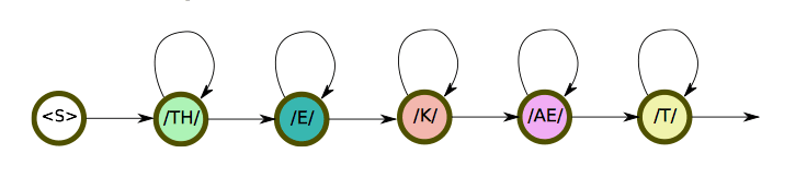
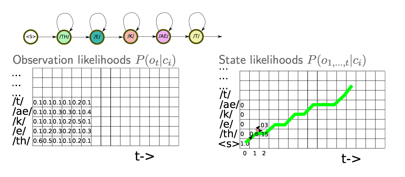
We model this with a Hidden Markov Model.

The system has a set of discrete states, transitions from state to state according to transition probabilities (Markovian: memoryless)
Acoustic observation when making a transition is conditioned on state alone. \(P(o_t|c_t)\)
We seek to recover the state sequence and consequently the phoneme sequence and consequently the word sequence.

We choose the decoder output as the most likely sequence \(\hat{w}\) from all possible sequences, \(Σ∗\), for an observation sequence \(o\): \[ \begin{align} \hat{w} & = \arg\max_{w\in\sum*}P(w|o) \\ & = \arg\max_{w\in\sum*}P(o|w)P(w) \\ \end{align} \] A product of Acoustic model and Language model scores. \[ P(o|w) = \sum_{d,c,p}P(o|c)P(c|p)P(p|w) \] Where \(p\) is the phone sequence and \(c\) is the state sequence.

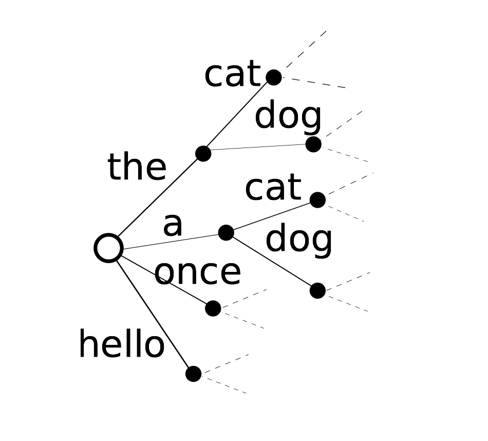
We can model word sequences with a language model: \[ P(w_1, w_2, ..., w_N) = P(w_0)\prod P(w_i|w_0, ..., w_{i-1}) \] Speech recognition as transduction

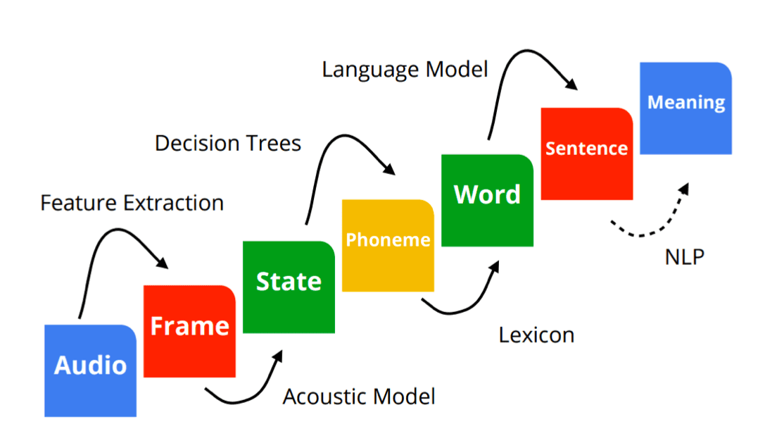
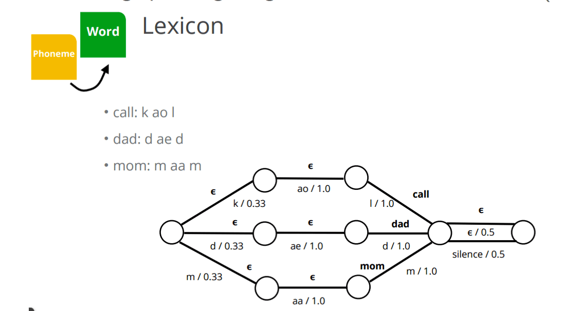
Lexicon: phoneme to word

Construct graph using Weighted Finite State Transducers (WFST).

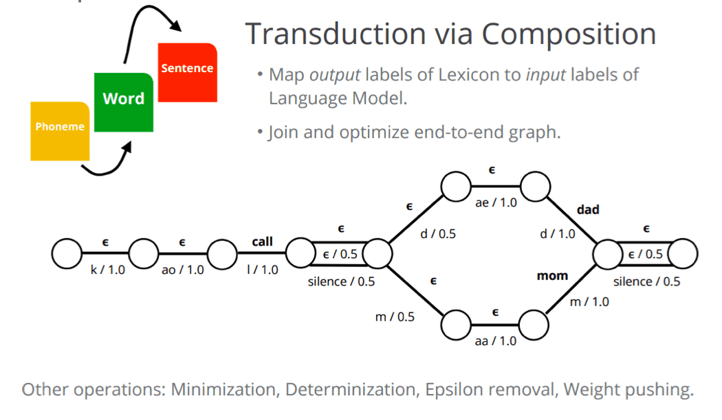
Compose Lexicon FST with Grammar FST \(L \circ G\).

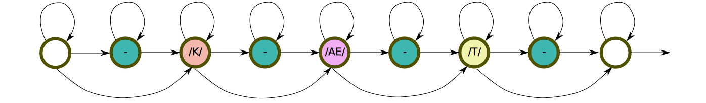
Phonetic Unites

Phonemes: “cat” → /K/, /AE/, /T/
Context independent HMM states \(k1, k2...\)
Context dependent states
Context dependent phones
Diphones (pairs of half-phones)
Syllables
Word-parts cf Machine translation (Wu et al., 2016)
Characters (graphemes)
Whole words Sak et al. (2014a, 2015); Soltau et al. (2016)
- Hard to generalize to rare words

Choice depends on language, size of dataset, task, resources available.

The difference between Phone and Phoneme

A phoneme is the smallest structural unit that distinguishes meaning in a language. Phonemes are not the physical segments themselves, but are cognitive abstractions or categorizations of them.

On the other hand, phones refer to the instances of phonemes in the actual utterances - i.e. the physical segments.

For example:

the words "madder" and "matter" obviously are composed of distinct phonemes; however, in american english, both words are pronounced almost identically, which means that their phones are the same, or at least very close in the acoustic domain.

Context dependent phonetic clustering

A phone’s realization depends on the preceding and following context, could improve discrimination if we model diﬀerent contextual realizations separately:

AE preceded by K, followed by T: AE+T-K

But, if we have 42 phones, and 3 states per phone, there are \(3 × 42^3\) context-dependent phones, But most of these won't be observed.

So cluster – group together similar distributions and train a joint model. Have a “back-oﬀ” rule to determine which model to use for unobserved contexts. Usually a decision tree.

Gaussian Mixture Models (GMM)

Dominant paradigm for ASR from 1990 to 2010

Model the probability distribution of the acoustic features for each state: \[ P(o_t|c_i) = \sum_j w_{ij}N(o_t;\mu_{ij}, \sigma_{ij}) \] Often use diagonal covariance Gaussians to keep number of parameters under control.

Train by the E-M algorithm (Dempster et al., 1977) alternating:

M: forced alignment computing the maximum-likelihood state sequence for each utterance
E: parameter \((µ, σ)\) estimation

Complex training procedures to incrementally ﬁt increasing numbers of components per mixture.

More components, better ﬁt. 79 parameters / component.

Given an alignment mapping audio frames to states, this is parallelizable by state. But hard to share parameters / data across states.

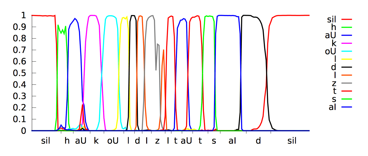
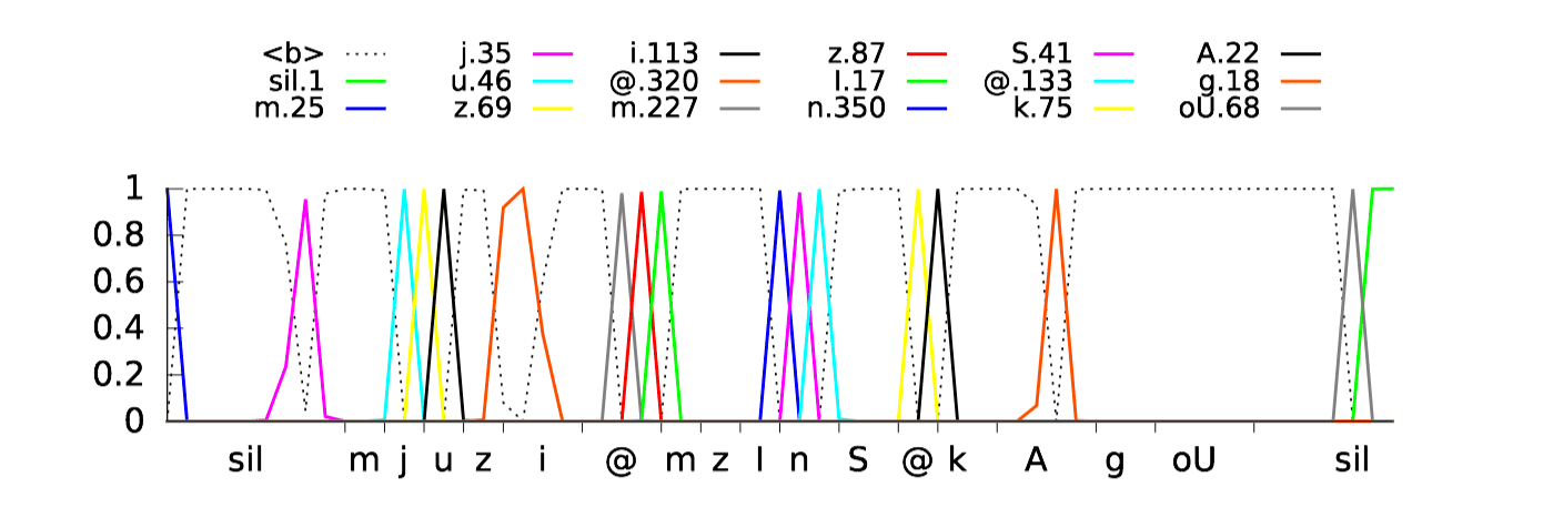
Forced alignment

Forced alignment uses a model to compute the maximum likelihood alignment between speech features and phonetic states. For each training utterance, construct the set of phonetic states for the ground truth transcription. Use Viterbi algorithm to ﬁnd ML monotonic state sequence under constraints such as at least one frame per state. Results in a phonetic label for each frame, which can give hard or soft segmentation.

With a transducer with states \(ci\):

Compute state likelihoods at time \(t\): \[ P(o_{1, ...., t}|c_i) = \sum_j P(o_t|c_j)P(o_{1, ..., t}|c_j)P(c_j|c_i) \] With transition probabilities: \(P(c_i|c_j)\), find the best path: \[ P(o_{1, ..., t}|c_i) = \max_j P(o_t|c_j)P(o_{1, ..., t}|c_j)P(c_i|c_j) \] I do not quite understand the image below actually:

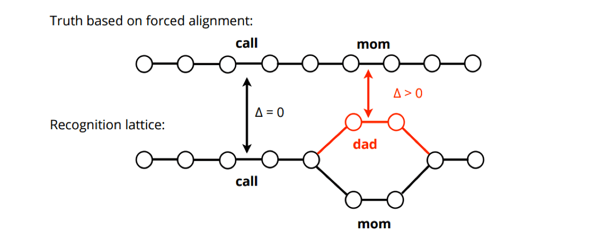
Decoding

Speech recognition unfolds in much the same way. Now we have a graph instead of a straight-through path.

Optional silences between words
Alternative pronunciation paths.

Typically use max probability, and work in the log domain. Hypothesis space is huge, so we only keep a “beam” of the best paths, and can lose what would end up being the true best path.

Neural network speech recognition

Two main paradigms

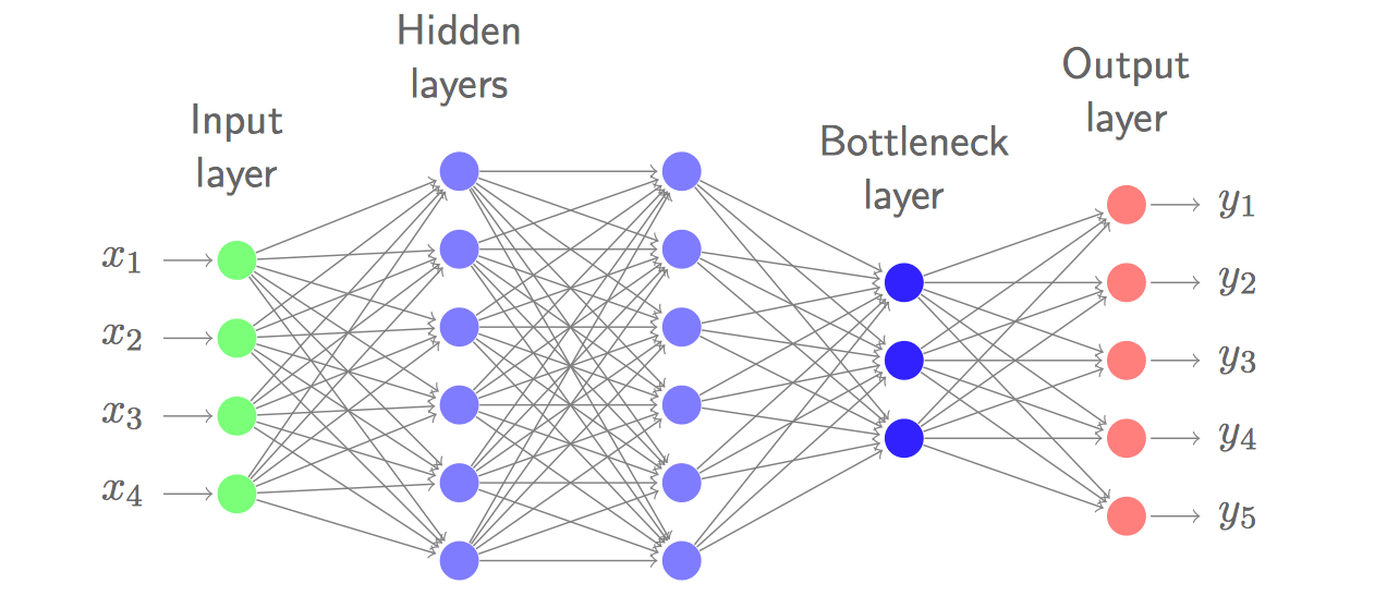
Use neural networks to compute nonlinear feature representations.
- “Bottleneck” or “tandem” features (Hermansky et al., 2000)
- Low-dimensional representation is modelled conventionally with GMMs.
- Allows all the GMM machinery and tricks to be exploited.
Use neural networks to estimate phonetic unit probabilities.

Neural network features

Train a neural network to discriminate classes. Use output or a low-dimensional bottleneck layer representation as features.

TRAP: Concatenate PLP-HLDA features and NN features.
Bottleneck outperforms posterior features (Grezl et al., 2007)
Generally DNN features + GMMs reach about the same performance as hybrid DNN-HMM systems, but are much more complex.

Hybrid neural networks

Train the network as a classiﬁer with a softmax across the phonetic units. Train with cross-entropy. Softmax will converge to posterior across phonetic states: \(P(c_i|o_i)\).

Now we model \(P(o|c)\) with a Neural network instead of a Gaussian Mixture model. Everything else stays the same. \[ P(o|c) = \prod_{t}P(o_t|c_t) \]

\[ \begin{align} P(o_t|c_t) & = \frac{P(c_t|o_t)P(o_t)}{P(c_t)} \\ & \varpropto \frac{P(c_t|o_t)}{P(c_t)} \\ \end{align} \]

For observations \(o_t\) at time \(t\) and a CD state sequence \(c_t\). We can ignore \(P(o_t)\) since it is the same for all decoding paths.

The last term is called the “scaled posterior”: \[ \log P(o_t|c_t) = \log P(c_t|o_t) - \alpha \log P(c_t) \] Empirically (by cross validation) we actually ﬁnd better results with a “prior smoothing” term \(α ≈ 0.8\).

Input features

Neural networks can handle high-dimensional features with correlated features. Use (26) stacked ﬁlterbank inputs. (40-dimensional mel-spaced ﬁlterbanks).

Example ﬁlters learned in the ﬁrst layer of a fully-connected network:

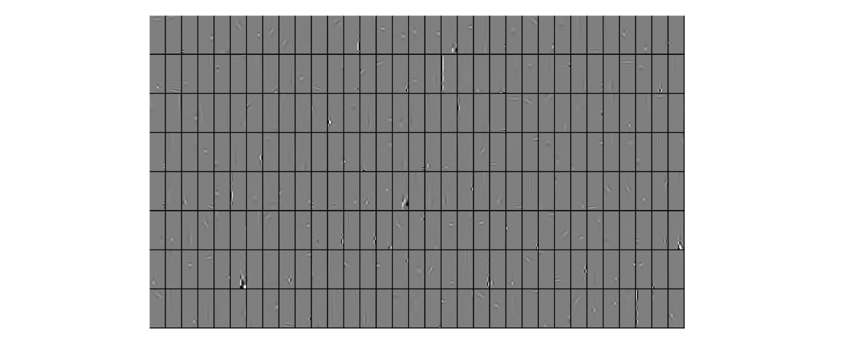
(33 x 8 ﬁlters. Each subimage 40 frequency vs 26 time.)

Network architectures

Fully connected
CNN
- Time delay neural networks
  - Waibel et al. (1989)
  - Dilated convolutions
- CNNs in time or frequency domain. Abdel-Hamid et al. (2014); Sainath et al. (2013)
- Wavenet (van den Oord et al., 2016)
RNN
- RNN (Robinson and Fallside, 1991)
- LSTM Graves et al. (2013)
- Deep LSTM-P Sak et al. (2014b)
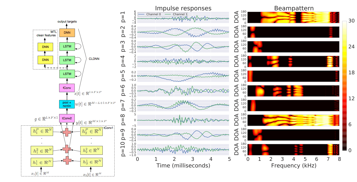
- CLDNN (right) (Sainath et al., 2015a)
- GRU. DeepSpeech 1/2 (Amodei et al., 2015)
- Bidirectional (Schuster and Paliwal, 1997) helps, but introduces latency.
- Dependencies not long at speech frame rates (100Hz).
- Frame stacking and down-sampling help.

Human parity in speech recognition (Xiong et al., 2016)

Ensemble of BLSTMs
i-vectors for speaker normalization
- i-vector is an embedding of audio trained to discriminate between speakers. (Speaker ID)
Interpolated n-gram + LSTM language model.
5.8% WER on SWB (vs 5.9% for human).

Traning losses

Cross Entropy Training

GMMs were trained with Maximum Likelihood
Conventional training uses Cross-Entropy loss. \[ L_{X\ ENT}(o_t, \theta) = \sum_{i=1}^Ny_t(i)\log\frac{y_t(i)}{\hat{y_t}(i)} \]
With large data we can use Viterbi (binary) targets: \(y_t ∈ {0, 1}\)
- − i.e. a hard alignment.
Can also use a soft (Baum-Welch) alignment (Senior and Robinson, 1994)

Connectionist Temporal Classiﬁcation (Graves et al., 2006)

CTC is a bundle of alternatives to conventional system:

CTC introduces an optional blank symbol between the ”real” labels.
Simple to implement in the FST framework
Continuous realignment — no need for a bootstrap model
Always use soft targets.
Don’t scale by posterior.
Similar results to conventional training.

Sequence discriminative training

Conventional training uses Cross-Entropy loss

Tries to maximize probability of the true state sequence given the data.

We care about Word Error Rate of the complete system. Design a loss that’s diﬀerentiable and closer to what we care about.

Applied to neural networks (Kingsbury, 2009).
Posterior scaling gets learnt by the network.
Improves conventional training and CTC by 15% relative.
bMMI, sMBR(Povey et al., 2008)

\[ P(S_r|X_r) = \frac{p(X_r, S_r)}{\sum_S p(X_r, S)} = \frac{p(X_r|S_r)P(S_r)}{\sum_Sp(X_r|S)P(S)} \]

\[ L_{mmi}(\theta) = -\sum_{r=1}^R\log P(S_r|X_r) \]

New architectures

Seq2seq

Basic sequence2sequence not that good for speech

Utterances are too long to memorize
Monotonicity of audio (vs Machine Translation)

Models

Attention + seq2seq for speech (Chorowski et al., 2015)
Listen, Attend and Spell (Chan et al., 2015)

Output characters until EOS, incorporates language model of training set. Harder to incorporate a separately-trained language model. (e.g. trained on trillions of tokens)

Watch, Listen, Attend and Spell (Chung et al., 2016)

Apply LAS to audio and video streams simultaneously.

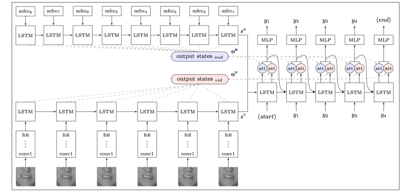
Train with scheduled sampling (Bengio et al., 2015)

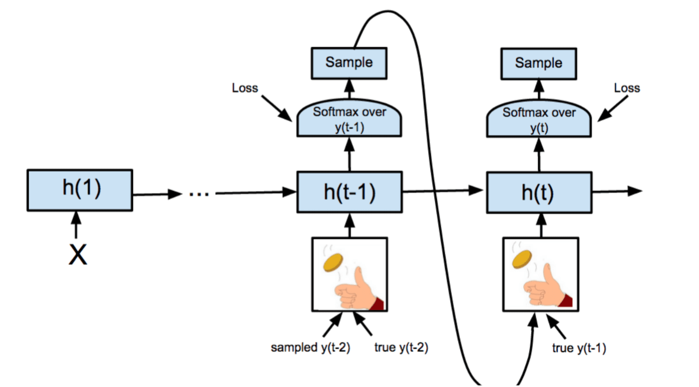
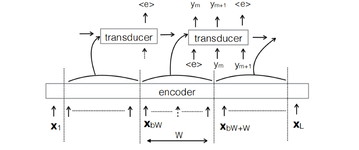
Neural transducer (Jaitly et al., 2015)

Seq2seq models require the whole sequence to be available. Introduce latency compared to unidirectional.

Solution: Transcribe monotonic chunks at a time with attention.

Raw waveform speech recognition

We typically train on a much-reduced dimensional signal.

Would like to train end-to-end.
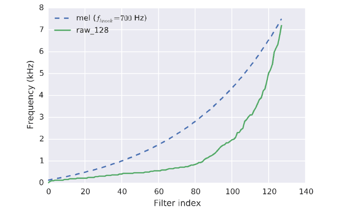
Learn ﬁlterbanks, instead of hand-crafting.

A conventional RNN at audio sample rate can’t learn long-enough dependencies.

Add a convolutional ﬁlter to a conventional system e.g. CLDNN (Sainath et al., 2015b)
WaveNet-style architecture
Clockwork RNN (Koutn´ık et al., 2014)
- Run a hierarchical RNN at multiple rates.

Frequency distribution of learned ﬁlters diﬀers from hand-initialization:

Speech recognition in noise

Multi-style training (“MTS”)
- Collect noisy data.
- Or, add realistic but randomized noise to utterances during training.
- e.g. Through a “room simulator” to add reverberation.
- Optionally add a clean-reconstruction loss in training.
Train a denoiser
NB Lombard eﬀect – voice changes in noise.

Multi-microphone speech recognition

Multiple microphones give a richer representation, “closest to the speaker” has better SNR.

Beamforming

Given geometry of microphone array and speed of sound
Compute Time Delay of Arrival at each microphone
Delay-and-sum: Constructive interference of signal in chosen direction.
Destructive interference depends on direction / frequency of noise.

More features for a neural network to exploit.

Important to preserve phase information to enable beam-forming

Factored multichannel raw waveform CLDNN (Sainath et al., 2016)